Linear Models
Model Overview
Model Synopsis
A linear model predicts the target as a weighted sum of the input features.
The independence and additivity of the model’s structure make it transparent. The weights communicate the global (with respect to the entire model) feature influence and importance.
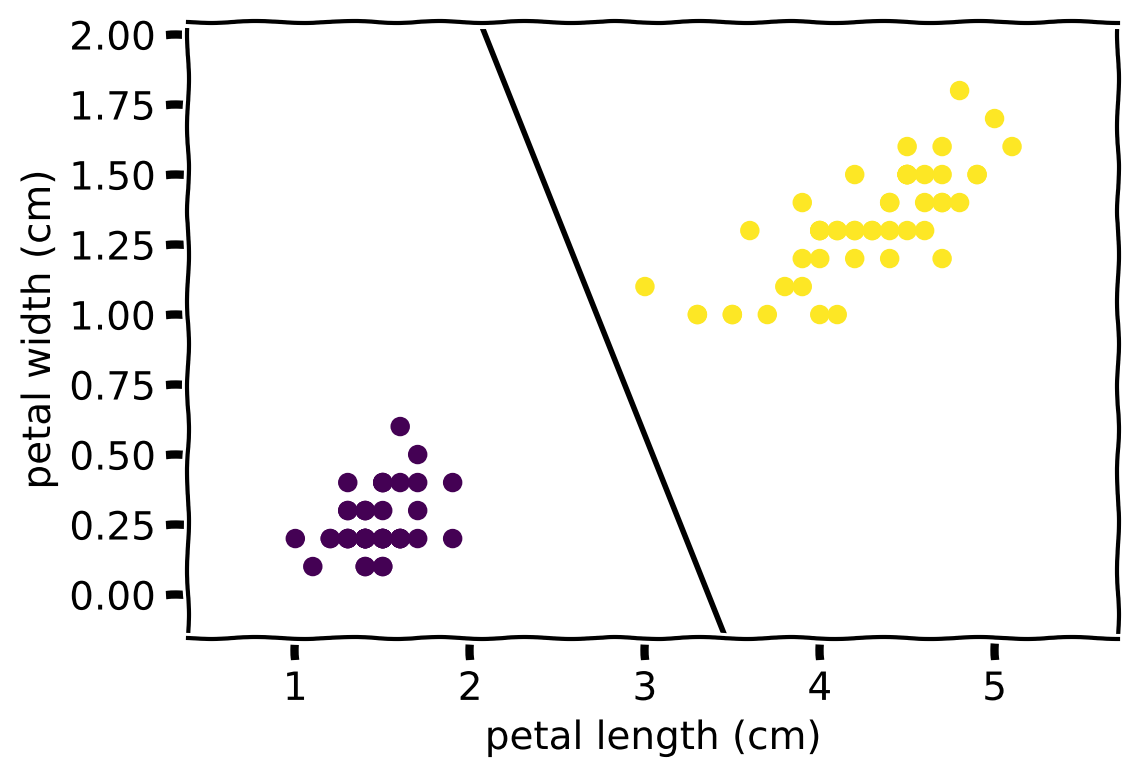
Toy Example
\[ f(\mathbf{x}) = -1.81 \;\; + \;\; 0.54 \times x_1 \;\; + \;\; 0.34 \times x_2 \]
\[\omega_0 = -1.81 \;\;\;\;\;\;\;\; \omega_1 = 0.54 \;\;\;\;\;\;\;\; \omega_2 = 0.34\]
Toy Example
Explanation Properties
| Property | Linear Models |
|---|---|
| relation | ante-hoc |
| compatibility | linear models |
| modelling | regression (crisp classification) |
| scope | global and local |
| target | model and prediction |
Explanation Properties
| Property | Linear Models |
|---|---|
| data | tabular |
| features | numerical and (one hot-encoded) categorical |
| explanation | model visualisation, feature influence & importance |
| caveats | feature correlation, target nonlinearity |
Examples
Model Visualisation
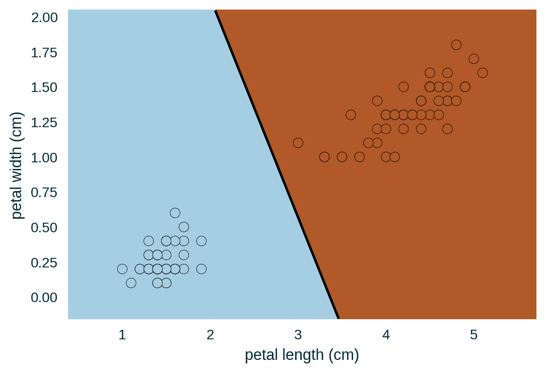
Model Equation
\[ f(\mathbf{x}) = -1.81 \;\; + \;\; 0.54 \times x_1 \;\; + \;\; 0.34 \times x_2 \]
\[\omega_0 = -1.81 \;\;\;\;\;\;\;\; \omega_1 = 0.54 \;\;\;\;\;\;\;\; \omega_2 = 0.34\]
Feature Influence & Importance
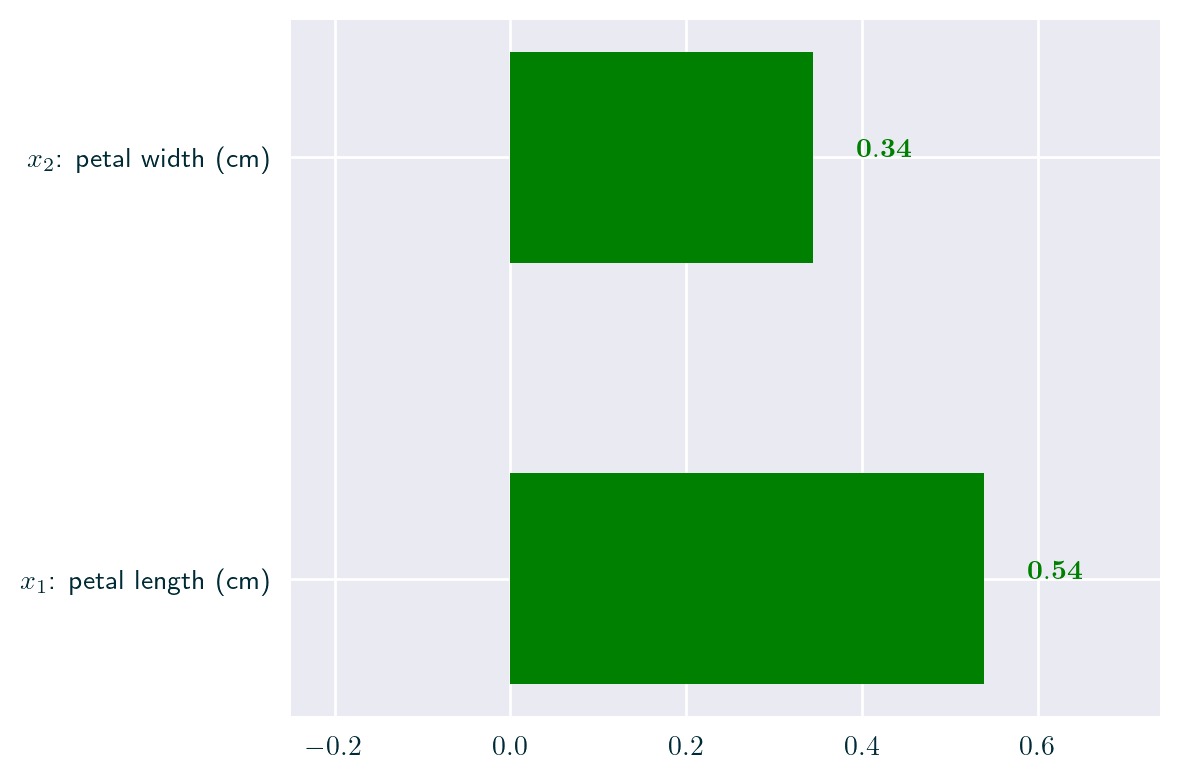
Feature Effect
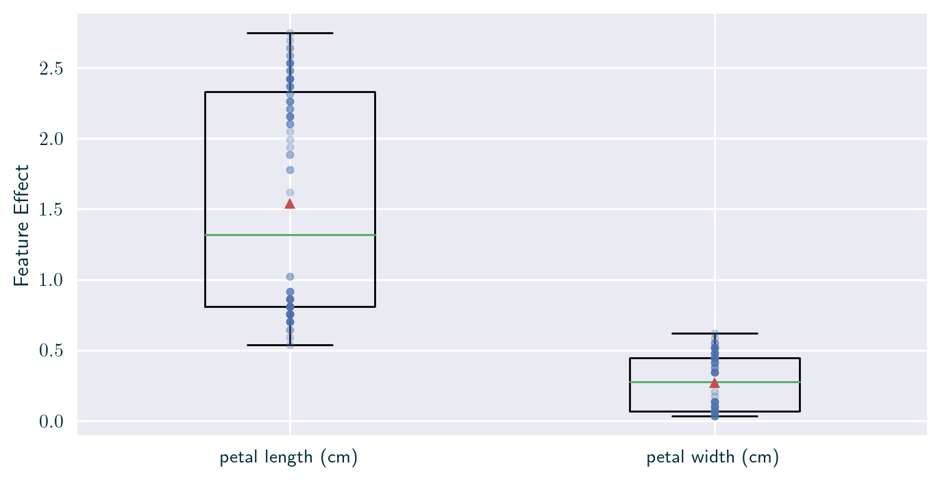
Feature Effect
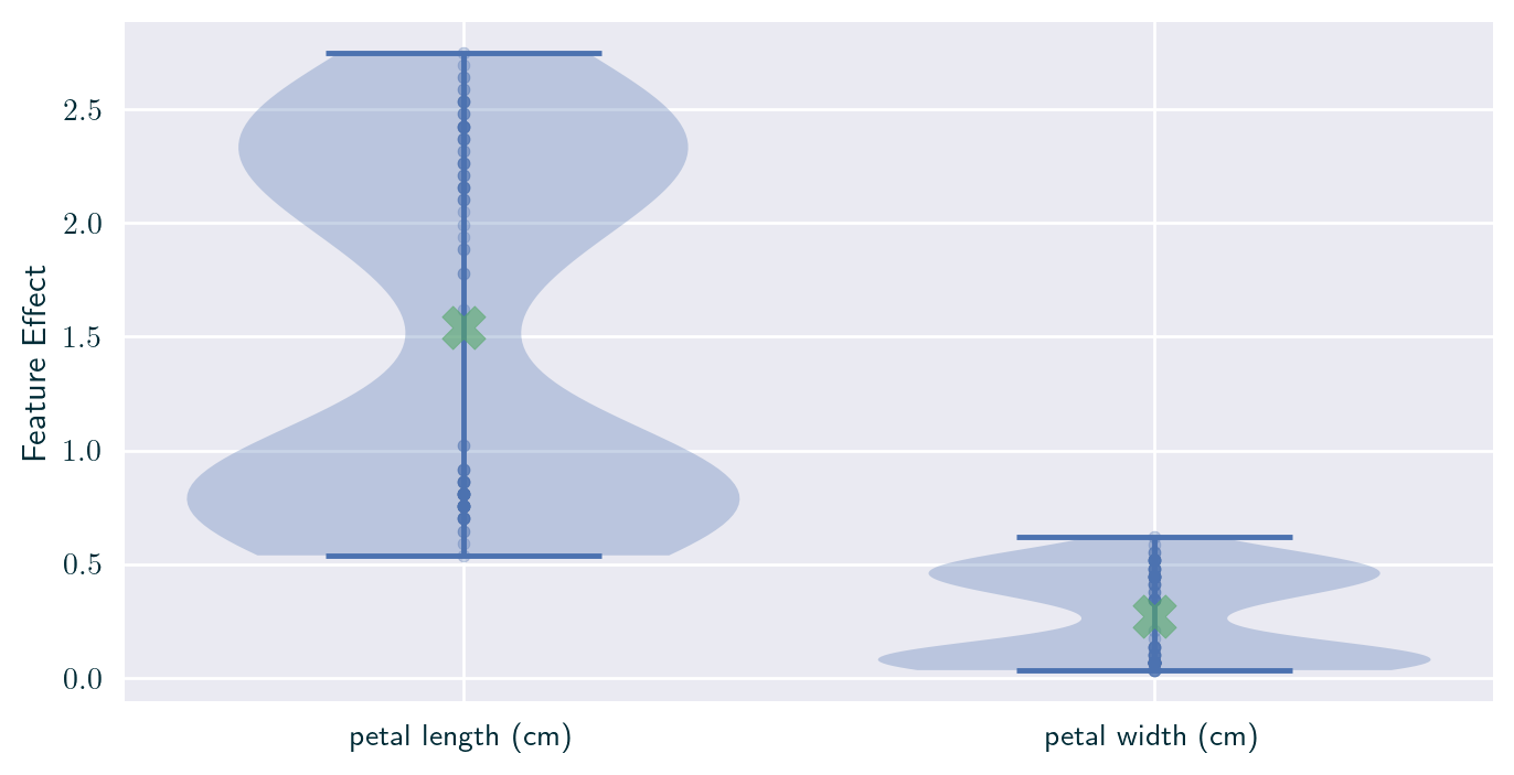
Individual Effect
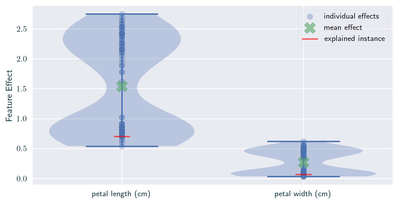
Individual Effect
\[\omega_0 = -1.81 \;\;\;\;\;\;\;\; \omega_1 = 0.54 \;\;\;\;\;\;\;\; \omega_2 = 0.34\]
\[x_1 = 1.30 \;\;\;\;\;\;\;\; x_2 = 0.20\]
Individual Effect
\[ f(\mathbf{x}) = -1.81 \;\; + \;\; \underbrace{0.54 \times 1.30}_{x_1} \;\; + \;\; \underbrace{0.34 \times 0.20}_{x_2} \]
\[ f(\mathbf{x}) = -1.81 \;\; + \;\; \underbrace{0.70}_{x_1} \;\; + \;\; \underbrace{0.07}_{x_2} \]
Individual Effect
Have you run `initjs()` in this notebook? If this notebook was from another user you must also trust this notebook (File -> Trust notebook). If you are viewing this notebook on github the Javascript has been stripped for security. If you are using JupyterLab this error is because a JupyterLab extension has not yet been written.
Textualisation
Increasing petal length (cm) by 1, increases the prediction by 0.54, ceteris paribus.
Increasing petal width (cm) by 1, increases the prediction by 0.34, ceteris paribus.
Variants
Feature Interaction
Manually introducing feature interaction terms allows linear models to account for such phenomena.
\[ f(\mathbf{x}) = \omega_0 + \omega_1 x_1 + \cdots + \omega_n x_n + \underbrace{\omega_{n+1} x_4 x_6}_{\textit{interaction}} \]
Generalized Linear Models
Generalized Linear Models (GLMs) allow to model alternative (to Gaussian) distributions of the prediction target.
\[ g(\mathbb{E}_Y(y|\mathbf{x})) = \omega_0 + \omega_1 x_1 + \cdots + \omega_n x_n \]
Generalized Additive Models
Generalized Additive Models (GAMs) allow to model nonlinear relationships – a weighted sum is replaced by a sum of arbitrary functions.
\[ g(\mathbb{E}_Y(y|\mathbf{x})) = \omega_0 + f_1(x_1) + \cdots + f_n(x_n) \]
Many More
This list is far from comprehensive and exhaustive.
Case Studies & Gotchas!
Feature Selection
- Large models may become overwhelming and incomprehensible (but still transparent)
- Achieved with feature selection or sparse linear models
\[ f(\mathbf{x}) = 0.2 \;\; + \;\; 0.25 \times x_1 \;\; - \;\; 0.47 \times x_2 \;\; + \;\; 0.01 \times x_3 \;\; + \;\; 0.70 \times x_4 \\ - \;\; 0.20 \times x_5 \;\; - \;\; 0.33 \times x_6 \;\; - \;\; 0.90 \times x_7 \]
Incomparability of Parameters
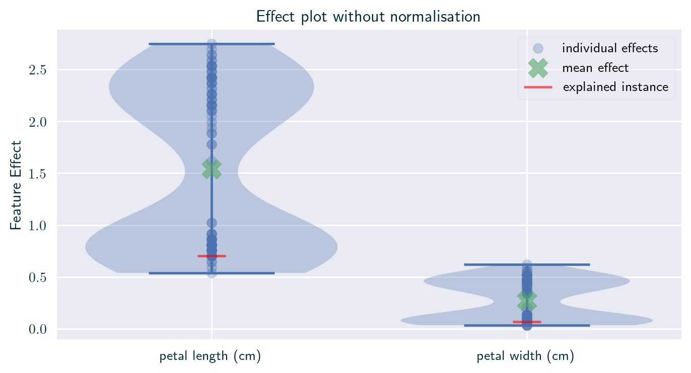
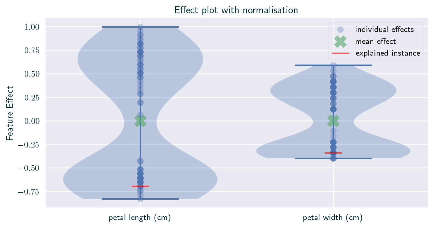
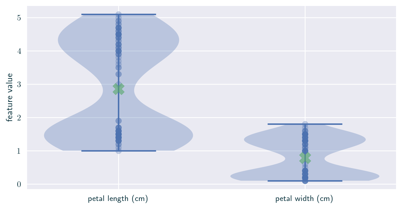
- The coefficients are uninformative unless the features are standardised (zero mean, one standard deviation) \[ \mathring{x}_i = \frac{x_i - \mu_i}{\sigma_i} \]
- The reference point becomes an all-zero instance – a mean-valued data point
- The intercept communicates the prediction of the reference point
Feasibility of the Reference Instance
The reference point may be out-of-distribution.
Incomparability of Parameters
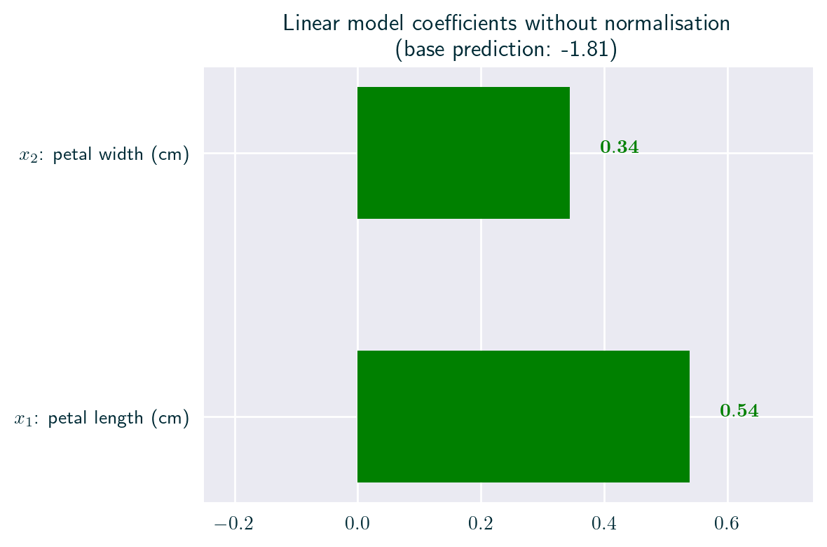
Incomparability of Parameters
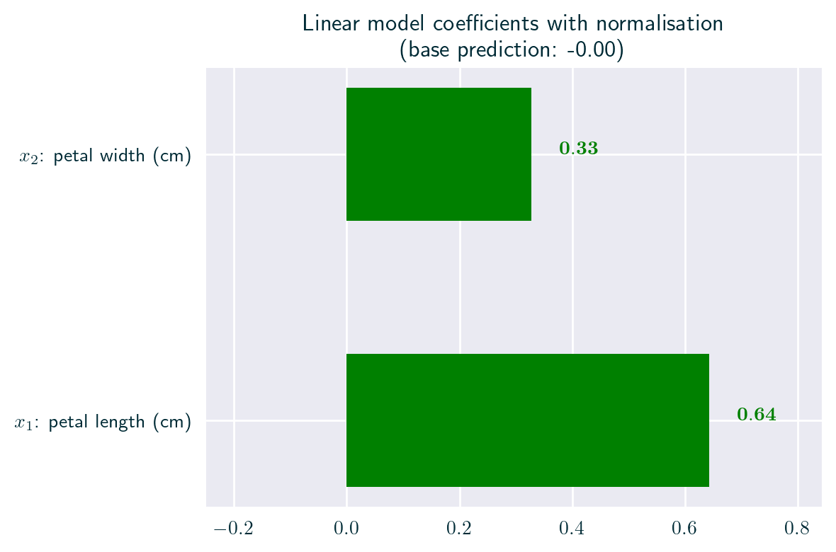
Incomparability of Parameters
Incomparability of Parameters
Incomparability of Parameters
Properties
Pros
- Transparent from the outset due to linearity – predictions are a linear combination of features
- Easy to interpret (given relevant background knowledge)
Cons
- Model linearity entails low complexity, but also low expressivity, hence low predictive power
- Feature interactions / correlations are not accounted for
- Poor modeling ability for nonlinear problems
- Decreased transparency for a large number of features (can be overcome with feature selection)
Caveats
- Interpretability is tricky without feature normalisation
- The interpretation based on unitary change in feature values ignores feature correlation and may lead to out-of-distribution instances
Further Considerations
Summary
- (Small) linear models are transparent
- Their interpretation should be viewed through their inherent limitations
Implementations
| Python | R |
|---|---|
| scikit-learn | built in |
Further Reading
- scikit-learn guide
- Interpretable Machine Learning book
- Machine learning: The art and science of algorithms that make sense of data textbook (Flach 2012)
Bibliography
Questions